Getting started
First, download the source code for the Matlab toolbox.
Source code is hosted on GitHub.
For more details about using the toolbox, see:
Getting_started.txt
How to use the GUI for indentation data analysis?
GUI stands for Graphical User Interface.
Create or update your personal YAML configuration file in the YAML folder
See here how to create / modify your YAML file…
Run the following Matlab script :
demo.m
Answer ‘y’ or ‘yes’ (or press ‘Enter’) to add the toolbox to the Matlab search path using this script:
path_management.m
The following window opens:

Figure 2 Screenshot of the main window of the NIMS toolbox.
Import your (nano)indentation results by clicking the ‘Select file’ button. Click here to have more details about valid format of data.
A load-displacement curve is plotted (with a power law fit). The loading work is also given in the title of the plot.
It is possible to plot the stiffness (raw data) without setting the GUI for Young’s modulus calculation.

Figure 3 File selector.

Figure 4 Plot of the load-displacement curve after loading of data.
Choose and set (if needed) the indenter used to obtain (nano)indentation data.
Select the lowest and the highest depth values (optional).
Set the CSM correction (Berkovich indenter only; optional).
Set the number of layers of your sample (0 = only bulk material, 1/2/3 = 1 to 3 thin layers on a substrate) (see Figure 5).

Figure 5 Convention used to define a multilayer specimen.
Set the thickness, the Poisson’s coefficient and the Young’s modulus to each layer.
Select the model to use for the contact displacement calculation and select the correction to apply.
Select ‘Red. Young’s modulus(film+sub)’ or ‘Red. Young’s modulus(film)’ in order to plot the evolution of the reduced Young’s modulus (raw calculation) of the sample vs. the evolution of the reduced Young’s modulus (modeled) of the sample and/or of the thin film.
Select the analytical bilayer or the multilayer model to use for the modelling of the reduced Young’s modulus of the top thin film.
Press the button ‘SAVE’ and a YAML results file and a picture of the figure (.png format) are created and stored in the following folder.
Press the button ‘FEM’ and generate a Python script to model nanoindentation of multilayer sample based on parameters used in the GUI for ABAQUS.

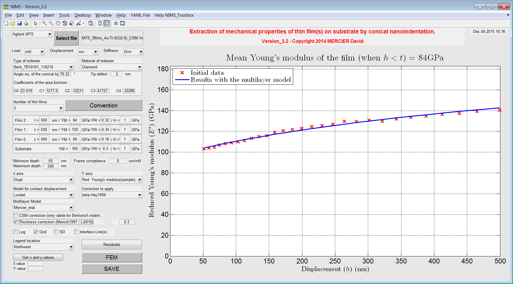
Figure 6 Plot of the evolution of the Young’s modulus of the sample with the elastic multilayer model as a function of the indentation depth.

Figure 7 Plot of the evolution of the Young’s modulus of the film with the elastic multilayer model as a function of the indentation depth.