Models for bulk material¶

The nanoindentation (or instrumented or depth sensing indentation) is a variety of indentation hardness tests applied to small volumes. During nanoindentation, an indenter is brought into contact with a sample and mechanically loaded.

The following parts give a short overview of models existing in the literature used for the extraction of mechanical properties of homogeneous bulk materials from indentation experiments with conical (sharp) indenters.

Please look at the ISO standard (ISO 14577 - 1 to 3), to perform nanoindentation tests on bulk material.

Some authors overviewed/reviewed already the nanoindentation technique :

Nanoindentation tests on bulk material¶

Conical indenters¶

The geometric properties of conical indenters are well described in [9].

Table 1 **Geometric properties of conical indenters.**¶
Indenter	Berkovich	Vickers	Cube-Corner	Conical
Shape	3-sided pyramid	4-sided pyramid	3-sided pyramid	Conical (angle \(\psi\))
Semi-angle from the apex	65.3°	68°	35.2644°	–
Equivalent cone angle	70.32°	70.2996°	42.28°	\(\psi\)
Projected Area	\(24.56h^2\)	\(24.504h^2\)	\(2.5981h^2\)	\(\pi{a_\text{c}}^2\)
Volume-depth relation	\(8.1873h^3\)	\(8.1681h^3\)	\(0.8657h^3\)	–
Projected area/face area	\(0.908\)	\(0.927\)	\(0.5774\)	–
Contact radius	–	–	–	\(htan\psi\)

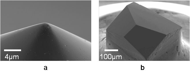
Figure 9 a) Conical indenter (45°) and b) Berkovich indenter.

These indenters have self-similar geometries which implies a constant strain and similarity of the stress fields.

Note

Indenters are mainly in diamond. Diamond has a Young’s modulus of 1070GPa and a Poisson’s ratio of 0.07 [9].

Load-Displacement curves¶

In this first part, only quasistatic (or monotonic) nanoindentation is considered, when a load is applied and removed to a sample. Parameters such as contact load \(F_\text{c}\) (in \(\text{N}\)) and depth of penetration (displacement) \(h_0\) (in \(\text{m}\)) are continuously recorded at a rapid rate (normally \(10\text{Hz}\)) during loading and unloading steps of the indentation test. Usually, the depth resolution is around the \(\text{nm}\)-level and the load resolution is around \(\text{nN}\)-level.

Initial penetration¶

The first correction step in nanoindentation testing is the determination of the initial contact point between the indenter and the sample [10].

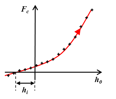
Figure 10 Schematic of the estimation of initial point.

Usually, the point of contact is determined from the load-displacement curve, when a sharp rise in the force signal is observed. Then, initial penetration \(h_\text{i}\) is estimated by extrapolating the recorded load–displacement data back to zero load.

(1)¶\[h = h_0 + h_\text{i}\]

With \(h\) the corrected penetration and \(h_0\) the recorded penetration.

A schematic of the load-displacement curve obtained from nanoindentation experiment after this first correction is given Figure 11.

The evolution of this curve depends on material properties of the sample and the indenter, and of the indenter’s geometry.

The tangent (or the slope) of the part of the unloading curve at the maximum load gives access to the contact stiffness \(S\) (in \(\text{N/m}\)):

(2)¶\[S = \frac{dF_\text{c}}{dh}\]

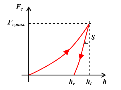
Figure 11 Schematic of indentation load-displacement curve.

With \(h_\text{t}\) the total penetration corrected of the frame compliance and \(h_\text{r}\) the residual indentation depth after unloading.

It is worth to mention that for quasistatic nanoindentation, the contact stiffness is a unique value obtained at the maximum load and at the maximum displacement. Nevertheless, it is possible to apply a multiple-point unload method, and then determine the contact stiffness for many indentation depths, in function of the number of points defined by the user (see Figure 12) [9].

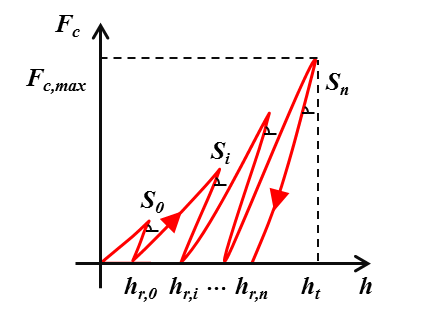
_images/load-disp_curve_multiplepoints.png

Figure 12 Schematic of indentation load-displacement curve with the multiple point unload method (here n points).

Frame compliance¶

Before any analysis, it is important to correct raw data of the effect of the frame compliance. The frame compliance is defined by the deflections of the load frame instead of displacement into the studied material. This frame compliance \(C_\text{f}\) (in \(\text{m/N}\)) contributes to the measured indentation depth and to the contact stiffness [10].

(3)¶\[h_\text{t} = h - F_\text{c}{C_\text{f}}\]

(4)¶\[S = \left(\frac{dh}{dF_\text{c}} - C_\text{f}\right)^{-1}\]

To determine the frame compliance, it is required to plot \(\frac{dh}{dF_\text{c}}\) vs. the corrected total depth \((1/h_\text{t})\) or the corrected plastic depth \((1/{h_\text{c}})\) (see the following part “Indentation contact topography” for the definition of the plastic depth) [8] and [10]. Then, a linear fit of this curve gives an intercept with the ordinate axis which is the frame compliance (see Figure 13).

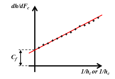
Figure 13 Schematic of the plot to determine the frame compliance.

It is advised to perform indentation tests on a variety of bulk standard specimens (fused silica, silicon and sapphire provide a very good range), in order to estimate better the frame compliance.

Moreover, when the sample flexes or has heterogeneities (free edges, interfaces between regions of different properties…), nanoindentation measurements are affected by the structural compliance \(C_\text{s}\). Then, it is possible to correct experimental data of this artifact by following the experimental approach proposed by [19].

Loading¶

Loubet et al. founded a good fit to the loading part of the load-displacement curve with a power-law relationship of the form [25] :

(5)¶\[F_\text{c} = K h_\text{t}^n\]

With \(K\) and \(n\) constants for a given material for a fixed indenter geometry.

It is possible to find in the litterature sometimes the following equation to fit the loading curve:

(6)¶\[F_\text{c} = K h_\text{t}^n + C\]

With \(C\) a constant which is used to account a small preload prior indentation testing [31].

Using the load-displacement curves analysis performed by Loubet et al., Hainsworth et al. proposed the following relationship to describe loading curves [16] :

(7)¶\[F_\text{c} = K h_\text{t}^2\]

With \(K\) a constant function of material properties (Young’s modulus and hardness) and the indenter.

In the same time, Giannakopoulos and Larsson established parabolic relationships between the load and the indentation depth, for purely elastic indentation of bulk materials with ideally Berkovich indenter (8) [22] and Vickers indenter (9) [12], by numerical studies.

(8)¶\[F_\text{c} = 2.1891 \left(1-0.21\nu -0.01{\nu}^2 -0.41{\nu}^3 \right) \frac{E}{1-{\nu}^2} h_\text{t}^2\]

(9)¶\[F_\text{c} = 2.0746 \left(1-0.1655\nu -0.1737{\nu}^2 -0.1862{\nu}^3 \right) \frac{E}{1-{\nu}^2} h_\text{t}^2\]

With \(\nu\) the Poisson’s ratio and \(E\) the Young’s modulus of the indented material.

Finally, it is first important to cite the work of Malzbender et al., who developped the relationship between the load and the indentation depth for elastoplastic materials, based on the knowledge of the Young’s modulus and the hardness values of the material [29]. Then, It is worth to mention the model of Oyen et al., who described sharp indentation behavior of time-dependent materials [34].

Unloading¶

Pharr and Bolshakov founded that unloading curves were well described by the following power-law relationship [36] :

(10)¶\[F_\text{c} = \alpha_\text{u} \left(h_\text{t} - h_\text{r}\right)^m\]

Where \(h_\text{r}\) is the final displacement after complete unloading, and \(\alpha_\text{u}\) and \(m\) are material constants. Many experiments performed by Pharr and Bolshakov leaded to an average value for \(m\) close to \(1.5\) for the Berkovich indenter.

Loading rate¶

The mechanical response of a material is function of the imposed indentation strain rate \(\dot{\epsilon}\) (in \(\text{s}^{-1}\)) [28]. Thus, it is meaningful to perform indentation tests with a constant indentation strain rate.

(11)¶\[\dot{\epsilon} = \frac{\dot{h}}{h} = \frac{1}{2} \frac{\dot{F_\text{c}}}{F_\text{c}}\]

Indentation contact topography¶

The indentation total depth is rarely equal to the indentation contact depth. Two kind of topography can occur:

the pile-up (indentation contact depth > indentation total depth) (see Figure 14 a and Figure 15);
the sink-in (indentation contact depth < indentation total depth) (see Figure 14 b).

The flow of material below the indenter is function of mechanical properties of the material.

Pile-up occurs when work-hardening coefficient is low (\(< 0.3\)) or if the ratio yield stress over Young’s modulus is less than \(1%\) [4], [5] and [7].

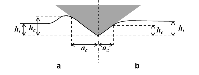
Figure 14 Schematic of indentation contact topography : a) “pile-up” and b) “sink-in”.

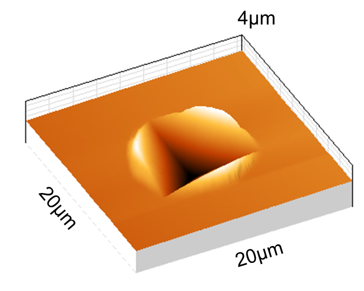
Figure 15 Residual topography of a Berkovich indent in PVD Gold thin film (500nm thick) with “pile-up” surrounding the indent, measured by atomic force microscopy.

Three main models defining the depth of contact \(h_\text{c}\) were developed to take into account this indentation contact topography.

Model of Doerner and Nix [8] :

(12)¶\[h_\text{c} = h_\text{t} - \frac{F_\text{c}}{S}\]

Model of Oliver and Pharr [32], [36] and [33] in case of sink-in:

(13)¶\[h_\text{c} = h_\text{t} - \epsilon \frac{F_\text{c}}{S}\]

Where \(\epsilon\) is a function of the indenter’s geometry (\(0.72\) for conical indenter, \(0.75\) for paraboloids of revolution and \(1\) for a flat cylindrical punch). An expression of \(\epsilon\) in function of the power law exponent \(m\) of the unloading curve fit has been proposed by Pharr et Bolshakov [36] :

\[\epsilon = m \left( 1 - \frac{ 2 \Gamma \left( \frac{m}{2(m-1)} \right)} {\sqrt[]{\pi} \Gamma \left( \frac{1}{2(m-1)}(m-1) \right)} \right)\]

With \(\Gamma\) a Matlab function which interpolates the factorial function : gamma.

Find here the Matlab function to plot the \(\epsilon\) function : epsilon_oliver_pharr.m.

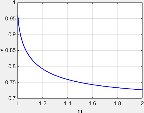
Figure 16 Evolution of epsilon in function of the power law exponent m of the unloading curve.

\(0.72\) should be most applicable for a Berkovich indenter, which is more like a cone than a paraboloid of revolution. But, Oliver and Pharr concluded after a large number of experiments that the best value for the Berkovich indenter is \(0.75\).

More recently, Merle et al. have found experimentally with indentation test in fused silica, a value of \(0.76\) for \(\epsilon\), which is in a good agreement with the literature for a paraboloid of revolution [30].

Model of Loubet et al. [18], [1] in case of pile-up:

(14)¶\[h_\text{c} = \alpha \left(h_\text{t} - \frac{F_\text{c}}{S} + h_0\right)\]

Where \(\alpha\) is a constant function of the indented material (usually around \(1.2\)) and the tip-defect \(h_0\).

Knowing the depth of contact, it is possible to determine the area of contact \(A_\text{c}\) (in \(\text{m}^{2}\)) for a perfect conical indenter (with a semi-angle from the apex \(\theta\)):

(15)¶\[A_\text{c} = \pi h_\text{c}^2 tan^2\left(\theta\right)\]

But, because conical indenters present imperfections and Berkovich or Vickers indenters are not perfectly conical, a general formulae of the contact area has been established by Oliver and Pharr [32], [33] :

(16)¶\[A_\text{c} = C_0 h_\text{c}^2 + \sum_{n=1}^8{C_\text{n} h_\text{c}^{1/2^{n-1}}}\]

With the coefficients \(C_0\) and \(C_\text{n}\) obtained by curve fitting procedures, from nanoindentation experiments in fused silica (amorphous and isotropic material).

For a perfect Berkovich indenter \(C_0\) is equal to \(24.56\) and for a perfect Vickers indenter \(C_0\) is equal to \(24.504\) (see Table 1).

The second term of the area function \(A_\text{c}\) describes a paraboloid of revolution, which approximates to a sphere at small penetration depths. A perfect sphere of radius \(R\) is defined by the first two terms with \(C_0 = -\pi\) and \(C_1 = 2 \pi R\). The first two terms also describe a hyperboloid of revolution, a very reasonable shape for a tip-rounded cone or pyramid that approaches a fixed angle at large distances from the tip.

An equivalent contact radius \(a_\text{c}\) (in \(\text{m}\)) is also defined based on the area function.

(17)¶\[a_\text{c} = \sqrt\frac{A_\text{c}}{\pi}\]

One other way to express the function area is that suggested by Loubet et al. [24], which describes a pyramid with a small flat region on its tip, the so-called tip defect (\(h_0\)). This geometry is described by the addition of a constant to the first two terms in (16).

Find here the Matlab function to calculate the contact depth, the function area and the contact radius: model_function_area.m.

Recently, in the paper of Yetna N’jock M. et al. [43], a criterion was proposed to forecast the behaviour during indentation experiments, following Giannakopoulos and Suresh methodology [13]. After analyzing either Vickers or Berkovich indentation tests on a wide range of materials, the following criterion is established \(\Delta\) :

(18)¶\[\Delta = \frac{h_\text{r}^{'}}{h_\text{t}^{'}}\]

With \(h_\text{r}^{'}\) and \(h_\text{t}^{'}\) residual contact depth and maximum depth after applying a compliance correction. Three preponderant deformation modes are distinguished :

\(\Delta = 0.83\) no deformation mode is preponderant;
\(\Delta < 0.83\) implies sink-in formation;
\(\Delta > 0.83\) implies pile-up formation.

Giannakopoulos and Suresh founded a critical value for a similar criterion about \(0.875\) [13].

Dynamic nanoindentation¶

The dynamic indentation is when a small dynamic oscillation (usually \(2\text{nm}\) of amplitude) with a given frequency (\(\omega\)) (usually \(45\text{Hz}\)) is imposed on the force (or displacement) signal. The amplitude of the displacement (or load) and the phase angle between the force and displacement signals (\(\phi\)) are measured using a frequency-specific amplifier. This technique allows to calculate the elastic stiffness and so the elastic properties continuously during the loading of the indenter [32], [23]. This technique is named Continuous Stiffness Measurement (CSM) for Agilent - MTS nanoindenter and Dynamic Mechanical Analysis (DMA) (using the CMX control algorithms) for Hysitron nanoindenter.

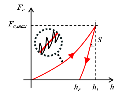
Figure 17 Schematic of the dynamic loading cycle.

(19)¶\[S = \left[\frac{1}{\frac{F_\text{c}}{h_\text{t}}\cos\phi-\left(K_\text{s} - m\omega^2\right)} - \frac{1}{K_\text{f}}\right]^{-1}\]

(20)¶\[C\omega = \frac{F_\text{c}}{h_\text{t}}\sin\phi - C_\text{s}\omega\]

With \(m\) the mass of the indenter column, \(C\) the harmonic contact damping in \(\text{N.s/m}\), \(C_\text{s}\) the system damping coefficient in \(\text{N.s/m}\), \(K_\text{s}\) the stiffness of the indenter support springs in \(\text{N/m}\) and \(K_\text{f}\) the stiffness of the load frame in \(\text{N/m}\).

Values \(m\), \(C_\text{s}\), \(K_\text{s}\) and \(K_\text{f}\) are function of the equipment used and are determined during calibration process.

This solution allows to determine the material properties as a continuous function of the indentation depth, but Pharr et al. have highlighted the influence of displacement oscillation on the basic measured quantities [37]. According to the authors, “the sources of the measurement error have their origin in the relative stiffness of the contact and its relation to the displacements that can be recovered during the unloading portion of the oscillation”. Based on that, the authors proposed the following corrections to determine the actual load (\(F_\text{c,act}\)), the actual displacement (\(h_\text{t,act}\)) and the actual stiffness (\(S_\text{act}\)):

(21)¶\[F_\text{c,act} = F_\text{c} + \frac{\Delta F_\text{c}}{2} = F_\text{c} + \sqrt{2}{\Delta F_\text{c,rms}}\]

(22)¶\[h_\text{t,act} = h_\text{t} + \frac{\Delta h_\text{t}}{2} = h_\text{t} + \sqrt{2} \Delta h_\text{t,rms}\]

(23)¶\[S_\text{act} = \frac{1}{\sqrt{2\pi}} \left(\frac{1}{K}\right)^\frac{1}{m} \left[1-\left(1-S{\frac{2\sqrt{2}{\Delta h_\text{t,rms}}} {F_\text{c,max}}}\right)^\frac{1}{m}\right]\frac{F_\text{c,max}}{{\Delta h_\text{t,rms}}}\]

With \(K\) and \(m\) constants determined from unloading curves. These constants are related by the following equation :

(24)¶\[K = \left(\frac{2}{{m\sqrt{\pi}}}\right)^m\]

Pharr and Bolshakov founded a value of \(1.380\) for \(m\) after many Berkovich indentation tests on a variety of materials [36]. Thus, a value of \(0.757\) is used for the constant \(K\), using (24).

Figure 18 Evolution of K in function of m.

Find here the Matlab function to calculate the corrections to apply on depth, load and stiffness during dynamic nanoindentation: CSM_correction.m.

Find here the Matlab function to calculate the constant \(K\) in function of \(m\): unload_k_m.m.

Extraction of elastic properties¶

Elastic properties of bulk material¶

Bulychev et al. [3] and Shorshorov M. K. et al. [39] were the first to determine the reduced Young’s modulus of a material with the relationships established by Love [26], Galin [11] and Sneddon [38], between the applied load and the displacement during an indentation test of an elastic material.

They proposed to expressed the reduced Young’s modulus \(E^{*}\) (in \(\text{GPa} = \text{N/m}^2\)) in function of the contact area and the contact stiffness :

(25)¶\[E^{*} = \frac{1}{2} \sqrt\frac{\pi}{A} S\]

Then, Oliver and Pharr [35], [32] democratized this formulae after introducing a correction factor identified by King [21] :

(26)¶\[E^{*} = \frac{1}{{2\beta}} \sqrt\frac{\pi}{A} S\]

With \(\beta\) a geometrical correction factor equal to :

\(1\) for circular indenters (e.g.: conical and spherical indenter);
\(1.034\) for three-sided pyramid indenters (e.g.: Berkovich indenter);
\(1.012\) for four-sided pyramid indenters (e.g.: Vickers indenter).

Woirgard has demonstrated analytically that the exact value of \(\beta\) for the perfectly sharp Berkovich indenter should be \(1.062\) [41].

Some authors proposed another correction factor function of the angle of the conical indenter and the Poisson’s ratio of the indented material [17] and [40]. For a conical indenter with an half-angle of \(\gamma \leq 60^{\circ}\) (e.g.: Cube-Corner indenter), the analytical approximation is :

(27)¶\[\beta = 1 + \frac{{\left(1-2\nu\right)}}{{4\left(1-\nu\right)tan\gamma}}\]

For a conical indenter with larger half-angle (e.g.: Berkovich indenter), the analytical approximation is :

(28)¶\[\beta = \pi{ \frac{\pi/4 + 0.1548cot\gamma{\frac{1-2\nu}{4\left(1-\nu\right)}}} {\left[\pi/2-0.8311cot\gamma{\frac{1-2\nu}{4\left(1-\nu\right)}}\right]^2}}\]

With \(\nu\) the Poisson’s ratio of the indented material.

Find here the Matlab function to plot the \(\beta\) function of Hay et al.: beta_hay.m.

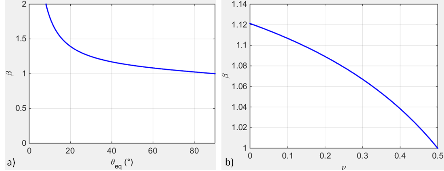
Figure 19 Plots of beta Hay : a) in function of the half-angle of the conical indenter (for a Poisson’s ratio of 0.3), and b) in function of the Poisson’s ratio for a Berkovich indenter.

Knowing the material properties of the indenter, it is possible to calculate the reduced Young’s modulus \(E^{'}\) (in \(\text{GPa} = \text{N/m}^2\)) of the indented material.

(29)¶\[\frac{1}{E^{'}} = \frac{1}{E^{*}} - \frac{1}{E_\text{i}^{'}}\]

(30)¶\[E = E^{'} \left(1-\nu^{2}\right)\]

(31)¶\[E_\text{i}^{'} = \frac{E_\text{i}}{\left(1-\nu_\text{i}^{2}\right)}\]

With \(\nu\) the Poisson’s ratio of the indented material and \(\nu_\text{i}\) the Poisson’s ratio of the material of the indenter.

Note

This method used to analyze indentation data is based on equations valid for isotropic homogeneous elastic solids.

Find here the Matlab function to calculate the Young’s modulus: model_elastic.m.

If dynamic nanoindentation is performed, a loss modulus \(E^{'*}\) (in \(\text{GPa} = \text{N/m}^2\)) can be defined by the following equation :

(32)¶\[E^{'*} = \frac{C\omega}{2} \sqrt\frac{\pi}{A}\]

Find here the Matlab function to calculate the loss modulus: loss_modulus.m.

Extraction of plastic properties¶

The hardness \(H\) (in \(\text{GPa} = \text{N/m}^2\)) of the material is defined according to Oliver and Pharr [32], by the following expression :

(33)¶\[H = \frac{F_\text{c,max}}{A_\text{c}}\]

Find here the Matlab function to calculate the hardness: model_hardness.m.

Energy approach¶

Another way to access indentation data is the use of the energy \(W_\text{tot}\) (in \(\text{J} = \text{N/m}\)) dissipated during the indentation. The elastic \(W_\text{e}\) and plastic \(W_\text{p}\) energies are respectively based on the integrals of the loading and unloading curves (see Figure 20) [6] and [29].

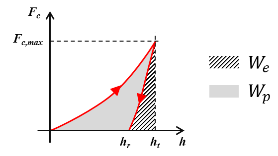
Figure 20 Schematic representation of indentation load–displacement curves with definition of different works of indentation.

(34)¶\[W_\text{tot} = \int_{0}^{h_\text{t}} {F_\text{c}\left(dh\right)}\]

(35)¶\[W_\text{e} = \int_{h_\text{r}}^{h_\text{t}} {F_\text{c}\left(dh\right)}\]

(36)¶\[W_\text{p} = W_\text{tot} - W_\text{e}\]

The “trapz” Matlab function is used to calculate the area below the load-displacement curve: trapz.m.

Methodology to extract properties without the function area¶

The ratio of the irreversible work \(W_\text{tot} - W_\text{e}\) to the total work \(W_\text{tot}\), appears to be a unique function of the Young’s modulus and the hardness of the material, independent of the work-hardening behavior [6].

(37)¶\[\frac{{W_\text{tot} - W_\text{e}}}{W_\text{tot}} = 1 - 5\frac{H}{E^{*}}\]

Then, combining the expression of the reduced Young’s modulus (26) with the expression of the hardness (33), leads to the following equation [20] and [33]:

(38)¶\[\beta \frac{4}{\pi} \frac{F_\text{c,max}}{S^2} = \frac{H}{E^{*}}\]

The \(\beta\) is initially not present in the equation given by [20].

These two last equations represent two independent relations that can be solved for \(H\) and \(E^{*}\) in a manner that does not directly involve the contact area.

The equation (38) is used as well to determine coefficients of the function area (16). Based on the assumption that the hardness and the Young’s modulus remain constant during indentation test in fused silica (isotropic material), the evolution of the ratio \(\frac{F_\text{c,max}}{S^2}\) should stay constant as well in function of the indentation depth.

More recently, Guillonneau et al. proposed a model to extract mechanical properties without using the indentation depth [14] and [15]. The method is based on the detection of the second harmonic for dynamic indentation testing. This model is interesting especially for penetration depths in the range of \(25\) to \(100\text{nm}\), where the uncertainties related to the displacement measurement disturb a lot.

References¶

[1]	Bec S. et al., “Improvements in the indentation method with a surface force apparatus” (2006).

[2]	Berkovich E.S., “Three-Faceted Diamond Pyramid for Studying Microhardness by Indentation” Zavodskaya Laboratoria 13(345) (1950).

[3]	Bulychev S.I. et al., “Determining Young’s modulus from the indentor penetration diagram.”, Zavod. Lab., 1973, 39, pp. 1137-1142.

[4]	Bolshakov A. and Pharr G.M., “Influences of pile-up on the measurement of mechanical properties by load and depth sensing indentation techniques.” (1998)

[5]	Cheng Y.T. and Cheng C.M. ,”Effects of ‘sinking in’ and ‘piling up’ on estimating the contact area under load in indentation.” (1998)

[6]	(1, 2) Cheng Y.T. and Cheng C.M. ,”Relationships between hardness, elastic modulus, and the work of indentation.” (1998)

[7]	Cheng Y.T. and Cheng C.M., “Scaling, dimensional analysis, and indentation measurements.” (2004)

[8]	(1, 2) Doerner M.F. and Nix W.D., “A method for interpreting the data from depth-sensing indentation instruments” (1986).

[9]	(1, 2, 3) Fischer-Cripps A.C., “Nanoindentation” Springer 3rd Ed. (2011).

[10]	(1, 2, 3) Fischer-Cripps A.C., “Critical review of analysis and interpretation of nanoindentation test data” (2006).

[11]	Galin L.A., “Spatial contact problems of the theory of elasticity for punches of circular shape in planar projection.”, J. Appl. Math. Mech. (PMM) (1946), 10, pp. 425-448.

[12]	Giannakopoulos A.E. et al., “Analysis of Vickers indentation” (1994).

[13]	(1, 2) Giannakopoulos A.E. and Suresh S., “Determination of elastoplastic properties by instrumented sharp indentation.” (1999).

[14]	Guillonneau G. et al.,”Extraction of mechanical properties with second harmonic detection for dynamic nanoindentation testing.” (2012).

[15]	Guillonneau G. et al.,”Determination of mechanical properties by nanoindentation independently of indentation depth measurement.” (2012).

[16]	Hainsworth S.V. et al., “Analysis of nanoindentation load-displacement loading curves.” (1996).

[17]	Hay J.C. et al., “A critical examination of the fundamental relations used in the analysis of nanoindentation data.” (1999).

[18]	Hochstetter G. et al., “Strain-rate effects on hardness of glassy polymers in the nanoscale range. Comparison between quasi-static and continuous stiffness measurements” (1999).

[19]	Jakes J.E. et al., “Experimental method to account for structural compliance in nanoindentation measurements” (2008).

[20]	(1, 2) Joslin D.L. and Oliver W.C., “A new method for analyzing data from continuous depth-sensing microindentation tests” (1990).

[21]	King R.B., “Elastic analysis of some punch problems for a layered medium” (1987).

[22]	Larsson P.-L. et al., “Analysis of Berkovich indentation” (1996).

[23]	Li X. and Bhushan B., “A review of nanoindentation continuous stiffness measurement technique and its applications.” (2002).

[24]	Loubet J.L. et al., “Vickers Indentation Curves of Magnesium Oxide (MgO).” (1984).

[25]	Loubet J.L. et al., “Vickers indentation curves of elastoplastic materials.” (1986).

[26]	Love A.E.H., “Boussinesq’s problem for a rigid cone.” (1939).

[27]	Lucca D.A. et al., “Nanoindentation: Measuring methods and applications” (2012).

[28]	Lucas B.N. et al., “Time Dependent Deformation During Indentation Testing.” (1996).

[29]	(1, 2) Malzbender J. and de With G., “Indentation load–displacement curve, plastic deformation, and energy.” (2002).

[30]	Merle B. et al., “Experimental determination of the effective indenter shape and e-factor for nanoindentation by continuously measuring the unloading stiffness.” (2012).

[31]	Morash K.R. and Bahr D.F., “An energy method to analyze through thickness thin film fracture during indentation.” (2007).

[32]	(1, 2, 3, 4, 5) Oliver W.C. and Pharr G.M., “An improved technique for determining hardness and elastic modulus using load and displacement sensing indentation experiments” (1992).

[33]	(1, 2, 3) Oliver W.C. and Pharr G.M., “Measurement of hardness and elastic modulus by instrumented indentation: Advances in understanding and refinements to methodology” (2004).

[34]	Oyen M.L. et al., “Load–displacement behavior during sharp indentation of viscous–elastic–plastic materials” (2003).

[35]	Pharr G.M. et al., “On the generality of the relationship among contact stiffness, contact area, and elastic modulus during indentation.” (1992).

[36]	(1, 2, 3, 4) Pharr G.M. and Bolshakov A., “Understanding nanoindentation unloading curves.” (2002).

[37]	Pharr G.M. et al., “Critical issues in making small-depth mechanical property measurements by nanoindentation with continuous stiffness measurement” (2009).

[38]	Sneddon I.N., “Boussinesqs problem for a rigid cone.” (1948).

[39]	Shorshorov M.K. et al., Sov. Phys. Dokl., 1982, 26.

[40]	Strader J.H. et al., “An experimental evaluation of the constant b relating the contact stiffness to the contact area in nanoindentation.” (2006).

[41]	Troyon M. and Lafaye S., “About the importance of introducing a correction factor in the Sneddon relationship for nanoindentation measurements” (2002).

[42]	VanLandingham M.R., “Review of Instrumented Indentation” (2003).

[43]	Yetna N’jock M. et al., “A criterion to identify sinking-in and piling-up in indentation of materials.” (2015).