Models for thin films
The following parts give a short overview of models existing in the literature used for the extraction of mechanical properties of thin films deposited on a substrate from indentation experiments with conical indenters.
Before everything, it is is worth to mention the work performed by Jennett N.M. and Bushby A.J. [24], about nanoindentation test on coatings, during the European project INDICOAT (SMT4-CT98-2249).
Progress from this project help in the development of the ISO standard (ISO 14577 - 1-4). The ISO 14577 - 4 is dedicated to nanoindentation on coatings.
- ISO 14577 - 1 , “Metallic materials – Instrumented indentation test for hardness and materials parameters – Part 1: Test method”, (2002).
- ISO 14577 - 2 , “Metallic materials – Instrumented indentation test for hardness and materials parameters – Part 2: Verification and calibration of testing machines”, (2002).
- ISO 14577 - 3 , “Metallic materials – Instrumented indentation test for hardness and materials parameters – Part 3: Calibration of reference blocks”, (2002).
- ISO 14577 - 4 , “Metallic materials – Instrumented indentation test for hardness and materials parameters – Part 4: Test method for metallic and non-metallic coatings”, (2007).
Some authors overviewed/reviewed already the nanoindentation technique applied to coatings :
- Pharr G.M. and Oliver W.C., “Measurement of Thin Film Mechanical Properties Using Nanoindentation” (1992).
- Menčík J. et al., “Determination of elastic modulus of thin layers using nanoindentation” (1997).
- Nix W.D., “Elastic and plastic properties of thin films on substrates: nanoindentation techniques” (1997).
- Van Vliet K.J. and Gouldstone A., “Mechanical Properties of Thin Films Quantified Via Instrumented Indentation” (2001).
- Šimůnková Š., “Mechanical properties of thin film–substrate systems” (2003).
- Bull S.J., “Nanoindentation of coatings” (2005).
- Fischer-Cripps, A.C., “Nanoindentation 3rd Ed.” (2011)
Nanoindentation tests on thin films
Composite reduced Young’s modulus and composite hardness
For indentation test on a coated specimen or on a multilayer sample (e.g.: thin films deposited on a substrate), the evolution of the Young’s modulus or the hardness calculated with models used for bulk materials, is function of the material properties and the thickness \(t\) (in \(\text{m}\)) of each underlying film (substrate included), and the properties and the geometry of the indenter.
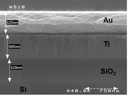
Figure 21 SEM cross-sectional observation of a multilayer sample.
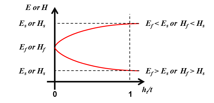
Figure 22 Typical evolution of Young’s modulus and hardness for a coated specimen in function of the normalized indentation depth.
Thus, the composite reduced Young’s modulus \(E^{'}\) and the composite hardness \(H\) calculated with the models used for bulk materials, can generally be expressed as a combination of respectively the reduced Young’s moduli \((E^{'}_\text{f})\) or the hardness \((H_\text{f})\) of each underlayer and respectively the reduced Young’s modulus \((E^{'}_\text{s})\) or the hardness \((H_\text{s})\) of the substrate. The reduced Young’s moduli and the hardness are in \(\text{GPa}\).
With \(i\) the indice of the layer and \(N\) the total number of layers.
Indentation contact topography
For nanoindentation tests on thin films, the contact topography is function of both thin film and substrate properties.
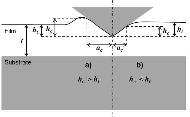
Figure 23 Schematic depiction of a) “pile-up” and b) “sink-in” observed during thin film indentation.
The Figure 23 a (“pile-up”) is typical of the case of a soft film on a hard substrate and the Figure 23 b (“sink-in”) of a hard film on a soft substrate [9]. The pile-up can be emphasized in case ot thin films, because of the material confinement by the substrate. To determine the depth of contact, the same models described for bulk material indentation are used.
Corrections to apply for thin film indentation
During nanoindentation tests of thin film on substrate, the thickness of the film beneath the indenter is smaller than its original value, because of plastic flow during loading. The use of the original film thickness \(t\) in the regression model cause a systematic shift or distortion of the Young’s modulus curve. A correction proposed by Menčík et al. can be applied, assuming a rigid substrate and determining the effective thickness \(t_\text{eff}\) (in \(\text{m}\)) [34], [45], [10], [2] and [32].
(41)¶\[\pi a^2 t_\text{eff} = \pi a^2 t - V\]
With \(V\) the volume displaced by the indenter and approximated by \(\pi a^2 h_\text{c} / 3\), for a conical indenter and contact depths \(h_\text{c}\) smaller than the film thickness.
(42)¶\[t_\text{eff} = t - \frac{h_\text{c}}{3}\]
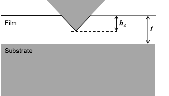
Figure 24 Indentation penetration of a thin film on a sample.
Recently, Li et al. proposed to express the local thinning effect as [32]:
(43)¶\[t_\text{eff} = t - \eta h_\text{c}\]
With \(\eta\) a parameter depending on the mechanical properties of the film and the substrate, and on the geometry of the indenter. Preliminary finite element calculations show that \(\eta\) should be independent of indentation depth and that its value ranges from \(0.3\) to \(0.7\) for materials that do not work harden.
Elastic properties of a thin film on a substrate
Several models to analyse indentation tests on bilayer sample and multilayer sample and to extract intrinsic material properties of the upper film (or the top coating) are detailed in the following part.
Some of the following models developed are detailed in the chapter 8 (“Nanoindentation of Thin Films”) of the book “Nanoindentation” written by A.C. Fischer-Cripps [15].
Bückle (1961)
Bückle proposed an empirical law (“rule of thumb”) to characterize thick coatings on a substrate [3]. It is possible to estimate the Young’s modulus of the coating for indentation depth lower than “\(10\text{%}\)” of the film thickness. But, because of the imperfections of the indenters, the roughness and the surface pollution, it is more meaningful to use this rule of the “\(10\text{%}\)”, for film thicker than \(500\text{nm}\).
Doerner and Nix (1986)
The model of Doerner and Nix is detailed in many papers [12], [29], [41] and [45], and is described by the following equation :
(44)¶\[\frac{1}{E^{'}} = \frac{1}{E_\text{f}^{'}} + \left(\frac{1}{E_\text{s}^{'}} - \frac{1}{E_\text{f}^{'}}\right) e^{-\alpha\left(x\right)}\]
With \(x=t/h_\text{c}\) and \(\alpha\) an empirically constant determined using the method of least squares.
The equation was modified by King [29] with the replacement of \(t/h_\text{c}\) by \(t/a_\text{c}\), and then by Saha and Nix [45] with the replacement of \(t/h_\text{c}\) by \((t-h_\text{c})/a_\text{c}\).
An empirical formulae based on the model of Doerner and Nix was proposed by Chen et al. in 2004 [10]:
(45)¶\[\frac{1}{E^{'}} = \frac{1}{E_\text{f}^{'}}\left[1-e^{-\alpha\left(x\right)^{(2/3)}}\right] + \frac{1}{E_\text{s}^{'}}e^{-\alpha\left(x\right)^{(2/3)}}\]
With \(x=t/h_\text{c}\) and \(\alpha\) an empirically constant determined using the method of least squares.
Find here the Matlab function for the Doerner and Nix model [12]: model_doerner_nix.m.
Find here the Matlab function for the Doerner and Nix model modified by King [29]: model_doerner_nix_king.m.
Find here the Matlab function for the Doerner and Nix model modified by Saha [45]: model_doerner_nix_saha.m.
Find here the Matlab function function for the Doerner and Nix model modified by Chen [10]: model_chen.m.
Gao et al. (1992)
The model of Gao is described by the following equation [16] :
(46)¶\[E^{'} = E^{'}_\text{s} + \left(E^{'}_\text{f} - E^{'}_\text{s}\right) \phi_{Gao_0}\left(x\right)\](47)¶\[\phi_{Gao_0} = \frac{2}{\pi} arctan \frac{1}{x} + \frac{1}{{2\pi\left(1-\nu_\text{c}\right)}} \left[\left(1-2\nu_\text{c}\right)\frac{1}{x}ln \left(1 + x^2 \right) - \frac{x}{{1+x^2}}\right]\](48)¶\[\nu_{c} = 1 + \left[{\frac{\left(1-\nu_\text{s}\right) \left(1-\nu_\text{f}\right)} {1-\left(1-\phi_{Gao_1}\right)\nu_\text{f} - \phi_{Gao_1}\nu_\text{s}}}\right]\]
With \(\nu_{c}\) the composite Poisson’s ratio, \(\nu_{s}\) the Poisson’s ratio of the substrate and \(\nu_{f}\) the Poisson’s ratio of the thin film.
(49)¶\[\phi_{Gao_1} = \frac{2}{\pi} arctan \frac{1}{x} + \frac{1}{{x\pi}}ln \left(1+x^2 \right)\]
With \(x=a_\text{c}/t\).
Find here the Matlab function for the weighting function \(\phi_{Gao_0}\) : phi_gao_0.m.
Find here the Matlab function for the weighting function \(\phi_{Gao_1}\) : phi_gao_1.m.
Find here the Matlab function for \(\nu_{c}\) the composite Poisson’s ratio : composite_poissons_ratio.m.
Find here the Matlab function for the Gao et al. model : model_gao.m.
Menčík et al. (1997)
Menčík et al. proposed the following structures to express the combination of \(E^{'}_\text{f}\) and \(E^{'}_\text{s}\) [34].
Where \(x\) is the ratio of the contact radius (\(a_\text{c}\)) or the contact depth (\(h_\text{c}\)), to the film thickness (\(t\)), and \(\phi\) and \(\psi\) are weight functions of the relative penetration \(x\). \(\phi\) is equal to \(1\) when \(x\) is equal to \(0\) and \(0\) when \(x\) is infinite.
Note
If the difference between Poisson’s ratio of the thin film and substrate is small, the values for uniaxial loading Young’s moduli, \(E\), \(E_\text{f}\), \(E_\text{s}\) can be used in previous equation.
Menčík et al. (linear model) (1997)
Menčík described too the linear model by the following expression [34] :
(52)¶\[E^{'} = E^{'}_\text{f} + \left(E^{'}_\text{s} - E^{'}_\text{f}\right)\left(x\right)\]
With \(x=a_\text{c}/t\).
Find here the Matlab function for the Menčík et al. linear function : model_menick_linear.m.
Menčík et al. (exponential model) (1997)
Menčík described the exponential model by the following expression [34] :
(53)¶\[E^{'} = E^{'}_\text{s} + \left(E^{'}_\text{f} - E^{'}_\text{s}\right) e^{-\alpha\left(x\right)}\]
With \(x=a_\text{c}/t\) and \(\alpha\) is an empirically constant determined using the method of least squares.
Find here the Matlab function for the Menčík et al. exponential function : model_menick_exponential.m.
Menčík et al. (reciprocal exponential model) (1997)
Menčík described the reciprocal exponential model by the following expression [34] :
(54)¶\[\frac{1}{E^{'}} = \frac{1}{E_\text{s}^{'}} + \left(\frac{1}{E_\text{f}^{'}} - \frac{1}{E_\text{s}^{'}}\right) e^{-\alpha\left(x\right)}\]
With \(x=a_\text{c}/t\) and \(\alpha\) is an empirically constant determined using the method of least squares.
Find here the Matlab function for the Menčík et al. reciprocal exponential function : model_menick_reciprocal_exponential.m.
Perriot et al. (2003)
The following system of equation describes the model developed by Perriot et al. [40] :
With \(x=a_\text{c}/t\), and \(k_0\) and \(n\) are adjustable constants determined using the method of least squares.
Find here the Matlab function for the Perriot et al. model : model_perriot_barthel.m.
Jung et al. (2004)
Jung et al. [27] have adapted for conical indentation of thin films, the simple empirical approach of Hu and Lawn [21] developed initially for spherical indentation on bilayer structures. The following power-law relationship allows the evaluation of the Young’s modulus of a thin film deposited on a substrate from nanoindentation experiments :
(57)¶\[E = E_\text{s} {\left(\frac{E_\text{f}}{E_\text{s}}\right)}^L\]
with \(L\) is the exponent term described by a dimensionless function :
(58)¶\[L = \frac{1}{\left[1+A{x}^B\right]}\]
With \(x=h_\text{c}/t\) and where \(A\) and \(B\) are adjustable coefficients.
Jung et al. founded \(A=3.76\) and \(B=1.38\) after regression fits of (57) to different data sets. These coefficients are not universal and need to be “calibrated” with experimental data or with finite element data for specified material systems.
Finally, to be more consistent with other analytical models implemented in this toolbox, the model of Jung is modified by using the reduced form of the Young’s moduli :
(59)¶\[E^{'} = E^{'}_\text{s} {\left(\frac{E^{'}_\text{f}}{E^{'}_\text{s}}\right)}^L\]
Find here the Matlab function for the sigmoidal function used in the Jung’s model : sigmoidal_jung.m.
Find here the Matlab function for the Jung et al. model : model_jung.m.
Bec et al. (2006)
The elastic model of Bec et al. is based on indentation by a rigid cylindrical punch (radius \(a_\text{c}\)) of a homogeneous film deposited on a semi-infinite half space [2].
This system is modelled by two springs connected in series :
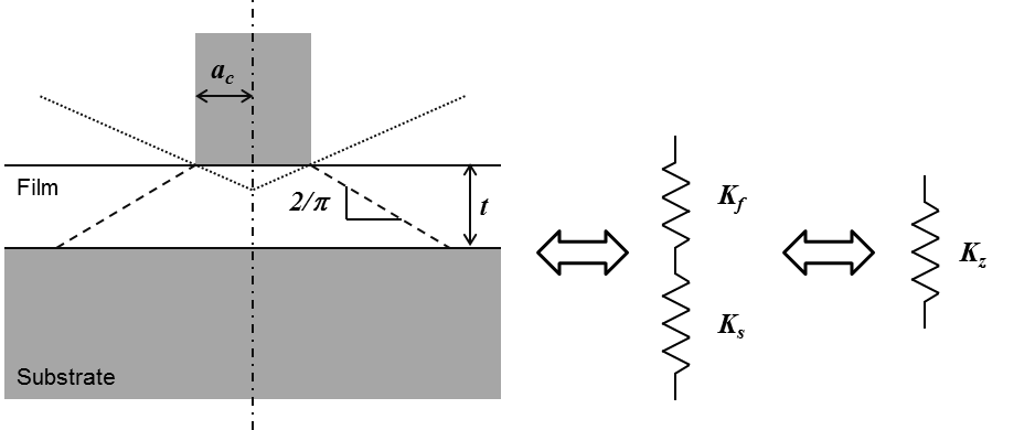
Figure 25 Schematic description of the bilayer model of Bec et al.
(60)¶\[K_\text{f} = \pi a_\text{c}^2 \frac{E^{'}_\text{f}}{t}\](61)¶\[K_\text{s} = 2 a_\text{c} E^{'}_\text{s}\](62)¶\[K_\text{z} = 2 a_\text{c} E^{'}\](63)¶\[\frac{1}{K_\text{z}} = \frac{1}{{f_\text{f}\left(a_\text{c}\right) K_\text{f}}} + \frac{1}{{f_\text{s}\left(a_\text{c}\right)K_\text{s}}}\](64)¶\[f_\text{f}\left(a_\text{c}\right) = f_\text{s}\left(a_\text{c}\right) = 1 + {\frac{2t}{\pi a_\text{c}}}\](65)¶\[\frac{1}{2 a_\text{c} E^{'}} = \frac{t}{\left(\pi a_\text{c}^2 + 2ta_\text{c}\right)E^{'}_\text{f}} + \frac{1}{2\left(a_\text{c} + \frac{2t}{\pi}\right)E^{'}_\text{s}}\]
Find here the Matlab function for the Bec et al. model : model_bec.m.
Korsunsky and Constantinescu (2009)
Korsunsky and Constantinescu proposed a simple model response function to the analysis of indentation of elastic coated systems [30] and [31]. They expressed the reduced Young’s modulus in terms of a linear law of mixtures of the form:
(66)¶\[E^{'} = E_\text{1}^{'} + \frac{E_\text{2}^{'} - E_\text{1}^{'}}{1 + \left(\frac{h_\text{t}}{\beta_{0}t}\right)^{\eta}}\]
Here \(E_\text{1}^{'}\), \(E_\text{2}^{'}\), \(\eta\) and \(\beta_{0}\) are positive constants to be determined from fitting. It may be expected that for very shallow indentation (\(\beta_{0} \ll 1\)), the corresponding parameter \(E_\text{1}^{'}\) ought to approach the Young’s modulus of the coating \(E_\text{f}^{'}\). Similarly, one might also expect that for very deep indentation (\(\beta_{0} \gg 1\)), the corresponding parameter \(E_\text{2}^{'}\) ought to approach the Young’s modulus of the substrate \(E_\text{s}^{'}\). Values of \(\eta\) and \(\beta_{0}\) depend on the indentation boundary condition, if the coating is a defined as a freely sliding layer or as a perfectly bonded layer.
Hay et al. (2011)
The present model of Hay et al. [19] is a development of the Song–Pharr model [44] and [48], which is already inspired by the Gao model [16].
(67)¶\[\frac{1}{\mu_\text{c}} = \left(1-\phi_{Gao_0}\right) \frac{1}{\mu_\text{s} + F\phi_{Gao_0}\mu_\text{f}} + \phi_{Gao_0}\frac{1}{\mu_\text{f}}\]
Where \(\mu_\text{c}\) (in \(\text{GPa} = \text{N/m}^2\)) is the composite shear modulus calculated from the composite Young’s modulus as :
(68)¶\[\mu_\text{c} = \frac{E}{2\left(1+\nu_\text{c}\right)}\]
Where \(\nu_\text{c}\) is the composite Poisson’s ratio given in Gao’s model.
(69)¶\[E = \left(1 - \nu_\text{c}^2\right)E^{'}\]
Knowing \(\mu_\text{c}\), it is possible to calculate \(\mu_\text{f}\) :
(70)¶\[\mu_\text{f} = \frac{-B + \sqrt{B^2-4AC}}{2A}\]
Where \(A = F \phi_{Gao_0}\)
(71)¶\[B = \mu_\text{s} - \left(F \phi_{Gao_0}^2 - \phi_{Gao_0} + 1\right)\mu_\text{c}\]
With \(F = 0.0626\), a constant obtained from finite element simulations.
Finally, the Young’s modulus of the film is calculated from the shear modulus and Poisson’s ratio of the film :
(74)¶\[E_\text{f} = 2\mu_\text{f}\left(1 + \nu_\text{f}\right)\]
Find here the Matlab function for the Hay et al. model : model_hay.m.
Bull (2014)
This model was originally proposed by Bull S.J. in 2011, in a paper about the mechanical characterization of ALD Alumina coatings [5]. Then, this simple method to determine the elastic modulus of a coating on a substrate using nanoindentation was developed in another paper in 2014 [6]. This model is based on the load support of a truncated cone of material beneath the indenter.
(75)¶\[E^{'} = \frac{F_\text{c}}{2a_\text{c}\left(h_\text{c} + h_\text{s} \right)}\](76)¶\[h_\text{c} = \frac{F_\text{c}}{\pi E_\text{f}} \left[ \frac{1}{a_\text{c} tan\alpha} - \frac{1}{a_\text{c} tan\alpha + t_\text{f} tan^2\alpha} \right]\](77)¶\[h_\text{s} = \frac{F_\text{c}}{\pi E_\text{s}} \left[ \frac{1}{a_\text{c} tan\alpha + t_\text{f} tan^2\alpha} - \frac{1}{a_\text{c} tan\alpha + (t_\text{f} + t_\text{s}) tan^2\alpha} \right]\]
Where \(E_\text{f}\) and \(E_\text{s}\) are the Young’s Modulus of the coating and substrate, \(t_\text{f}\) and \(t_\text{s}\) are the coating and substrate thickness, and \(\alpha\) is the semi-angle of the cone material which supports the load. In fact, by assuming that the material thickness is very much greater than the contact radius, it is possible to replace in the previous equation \(tan\alpha\) by \(2\pi = 32.48°\). Finally, by assuming that the substrate is very much thicker than the coating \((t_\text{s} >> t_\text{f})\), the equation (75) can be rewritten :
(78)¶\[E^{'} = \frac{1}{\frac{1}{E_\text{f}} \left[\frac{2t_\text{f}}{\pi a_\text{c} + 2t_\text{f}} \right] + \frac{1}{E_\text{s}} \left[\frac{\pi a_\text{c}}{\pi a_\text{c} + 2t_\text{f}} \right]}\]
This last equation from Bull S.J. is exactly the same as equation (65), proposed by Bec et al. in 2006, with a unique difference which is the use by Bull S.J. of the non reduced form of the Young’s moduli of the coating and the substrate.
Elastic properties of a thin film on a multilayer system
In 2008, Pailler-Mattei et al. proposed an extension of the Bec’s model to a bilayer system deposited on a substrate [39].
But more recently, Mercier et al. established a generalization of the Bec’s model to \(N+1\) layers sample.
Mercier et al. (2010)
The elastic model of Mercier et al. for a multilayer sample on \(N+1\) layers is an extension of the Bec et al. model [35] and [36].
With \(a_{\text{c},0}\) equal to \(a_{\text{c}}\).
Thus, the Young’s modulus of the film can be calculated as :
(81)¶\[E^{'}_{\text{f},0} = \left[\frac{\pi a_{\text{c},0}^2 + 2t_0a_{\text{c},0}}{t_0} \left[\frac{1}{2 a_{\text{c},0} E^{'}} - {\left(\sum_{i=1}^{N} {\frac{t_i}{\left(\pi a_{\text{c},i}^2 + 2t_ia_{\text{c},i}\right)E^{'}_{\text{f},i}} + \frac{1}{2\left(a_{\text{c},N} + \frac{2t_N}{\pi}\right)E^{'}_\text{s}}}\right)}\right]\right]^{-1}\]
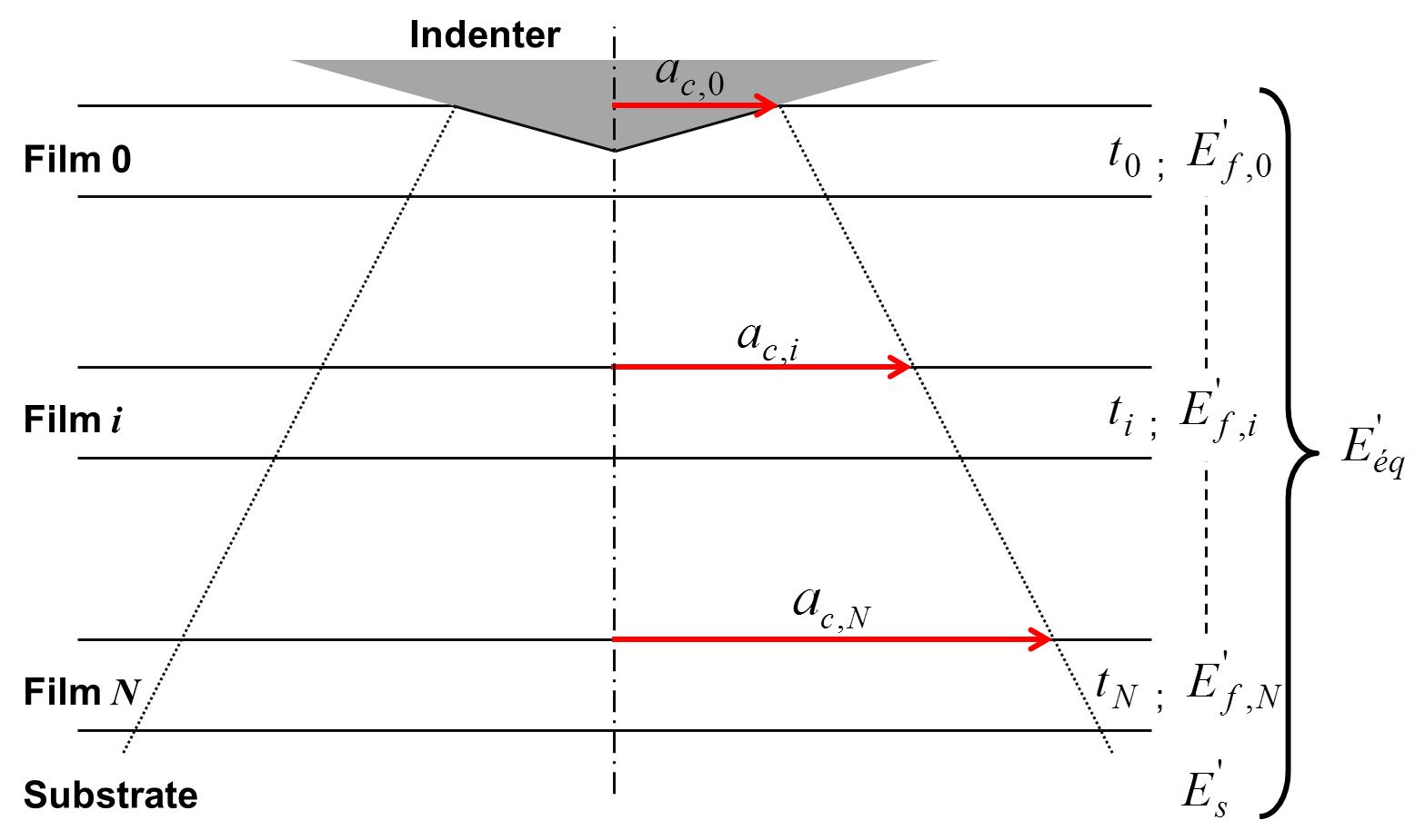
Figure 26 Schematic of elastic multilayer model.
It is advised to perform nanoindentation tests on each layer of the multilayer sample, from the substrate up to the final stack of layers (see Figure 27). By successive iterations using the model of Mercier et al., values of Young’s modulus of each layer are extracted from the contact stiffness.
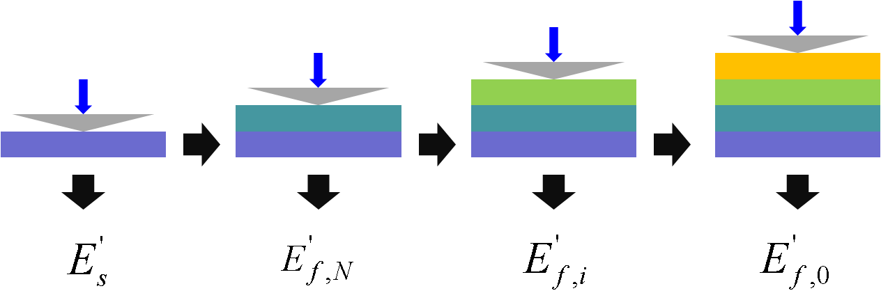
Figure 27 Experimental process to apply for elastic multilayer model.
Find here the Matlab function for the Mercier et al. model : model_multilayer_elastic.m.
Puchi-Cabrera et al. (2015)
Puchi-Cabrera et al. proposed in 2015, a description of the composite elastic modulus of multilayer coated systems [42], based on the physically-based concept advanced by Rahmoun et al. [43] :
(82)¶\[\frac{1}{E} = \sum_{i=1}^{N} {\frac{x^\text{i}_\text{v}}{E^\text{i}_\text{f}} + \frac{x^\text{s}_\text{v}}{E_\text{s}}}\]
With \(x^\text{i}_\text{v}\) and \(x^\text{s}_\text{v}\), respectively the volume fraction of each layer and the corresponding volume fraction of the substrate material. In his paper, Puchi-Cabrera modified and extended from the bilayer to the multilayer specimen, the models of Doerner and Nix, Gao, Bec, Menčík, Perriot and Barthel, Antunes, Korsunsky and Constantinescu and Bull.
Plastic properties of a thin film on a substrate
It is possible to estimate empirically the hardness of the coating for indentation depth lower than “\(40\text{%}\)” of the film thickness. Like the rule of the “\(10\text{%}\)” for the extraction of elastic properties, it is a “rule of thumb”. Because of the imperfections of the indenters, the roughness and the surface pollution, it is more meaningful to use this rule of the “\(40\text{%}\)”, for film thicker than \(500\text{nm}\).
Bückle (1961)
Bückle proposed an expression of the composite hardness \(H\) in the case of a two-layer material with a weighted sum of the different layer hardnesses during indentation process [3].
(83)¶\[H = aH_\text{f} + bH_\text{s}\]
With \(H_\text{f}\) the hardness of the film, \(H_\text{s}\) the hardness of the substrate and \(a + b = 1\). \(a\) varies from \(1\) when the hardness is not affected by the substrate, to \(0\) when the indentation depth is approaching the film thickness.
Kao and Byrne (1981)
Kao and Byrne proposed the following model to describe the evolution of the composite hardness in function of the reciprocal indentation depth [28], based on Bückle’s model [3] :
(84)¶\[H \simeq H_\text{s} + 2 k_1 t_\text{f}\left(H_\text{f} - H_\text{s} \right)\frac{1}{h}\]
With \(k_1\) a weighting factor of about 9%, independent of material characteristics.
Jönsson and Hogmark (1984)
Jönsson and Hogmark used a simple geometrical approach based on a area “law of mixtures” to separate the substrate and film contributions to the measured hardness from Vickers indentation [25].
(85)¶\[H = \frac{A_\text{f}}{A}H_\text{f} + \frac{A_\text{s}}{A}H_\text{s}\]
With \(A_\text{f}\) the area on which the mean pressure \(H_\text{f}\) acts and \(A_\text{s}\) the area on which the mean pressure \(H_\text{s}\) acts. The total area \(A\) is the sum of \(A_\text{f}\) and \(A_\text{s}\) and the following expressions for the area ratios are given by Jönsson and Hogmark:
With \(d\) the diagonal of the indent, \(t\) the film thickness and \(C\) a constant equal to \(0.5\) for hard coatings on very soft substrates (\(6.3 < \frac{H_\text{f}}{H_\text{s}} < 12.9\)) or to \(1\) when the coatings and substrate hardnesses are more similar (\(1.8 < \frac{H_\text{f}}{H_\text{s}} < 2.3\)).
Burnett and Rickerby (1984)
Burnett and Rickerby proposed afterwards a model based on a “volume law of mixtures” similar to Jönsson’s relation, considering the volumes of the plastic zones, \(V_\text{f}\) and \(V_\text{s}\) respectively in the film and in the substrate [7] [8].
(88)¶\[H = \frac{V_\text{f}}{V}H_\text{f} + \frac{V_\text{s}}{V}H_\text{s}\]
With \(V = V_\text{f} + V_\text{s}\).
Saha and Nix (2002)
Based on the methodology proposed by Joslin and Oliver (1990) [26] for a bulk material, extended to the coated system by Page et al. [38], Saha and Nix proposed to use the following equation, giving the evolution of the hardness in function of indentation depth, even when pile-up occurs [45]:
With \(x=(t-h_\text{c})/a_\text{c}\) and \(E_\text{i}^{'}\) the reduced Young’s modulus of the indenter.
This model was reused later by Han et al. [17] and [18].
Note
This model is valid only for the case of elastically inhomogeneous film/substrate systems.
Plastic properties of a thin film on a multilayer system
Engel et al. (1992)
Engel et al. proposed a simple method of interpreting the superficial (Vickers) hardness of multilayered specimen [13], by expanding the concept of Jönsson and Hogmark [25] :
With \(N\) the number of layers deposited on the substrate, \(A_\text{f,i}\) and \(H_\text{f,i}\) respectively the flow pressure area and the hardness of an intermediate layer. According to the author, this model is applicable as long as the ratio of the film thickness \(t_\text{f}\) over the indentation imprint size (i.e. the diagonal \(d\) of square imprint in case of Vickers indentation) is less than 0.2, resulting in a parallel displacement of indenter, layers, and substrate.
Rahmoun et al. (2009)
(93)¶\[H = \frac{A_\text{f}}{A}H_\text{f} + \frac{A_\text{i}}{A}H_\text{i} + \frac{A_\text{s}}{A}H_\text{s}\](94)¶\[\frac{A_\text{f}}{A} = \frac{2t_\text{f}}{h} - \frac{t_\text{f}^2}{h^2}\](95)¶\[\frac{A_\text{i}}{A} = \frac{2t_\text{f}}{h} - \frac{t_\text{i}^2}{h^2} - 2\frac{t_\text{i}t_\text{f}}{h^2}\](96)¶\[\frac{A_\text{s}}{A} = 1 - \frac{2(t_\text{f}+t_\text{i})}{h} + \frac{(t_\text{f}+t_\text{i})^2}{h^2}\]
References
| [1] | Arrazat B. et al., “Nano indentation de couches dures ultra minces de ruthénium sur or” (2010). |
| [2] | (1, 2) Bec S. et al., “Improvements in the indentation method with a surface force apparatus” (2006). |
| [3] | (1, 2, 3) Bückle H., “VDI Berichte” (1961). |
| [4] | Bull S.J., “Nanoindentation of coatings” (2005). |
| [5] | Bull S.J., “Mechanical response of atomic layer deposition alumina coatings on stiff and compliant substrates” (2011). |
| [6] | Bull S.J., “A simple method for the assessment of the contact modulus for coated systems.” (2014). |
| [7] | Burnett P.J. and Rickerby D.S., “The mechanical properties of wear-resistant coatings: I: Modelling of hardness behaviour.” (1987). |
| [8] | Burnett P.J. and Rickerby D.S., “The mechanical properties of wear-resistant coatings: II: Experimental studies and interpretation of hardness.” (1987). |
| [9] | Chen X. and Vlassak J.J., “Numerical study on the measurement of thin film mechanical properties by means of nanoindentation.” (2001). |
| [10] | (1, 2, 3, 4) Chen S. et al., “Nanoindentation of thin-film-substrate system: Determination of film hardness and Young’s modulus” (2004). |
| [11] | Chicot D. and Lesage J., “Absolute hardness of films and coatings” (1995). |
| [12] | (1, 2) Doerner M.F. and Nix W.D., “A method for interpreting the data from depth-sensing indentation instruments” (1986). |
| [13] | Engel P.A. et al., “Interpretation of superficial hardness for multilayer platings*” (1992). |
| [14] | Fernandes J.V. et al., “A model for coated surface hardness” (2000). |
| [15] | Fischer-Cripps, A.C., “Nanoindentation 3rd Ed.” (2011) |
| [16] | (1, 2) Gao H. et al., “Elastic contact versus indentation modeling of multi-layered materials” (1992). |
| [17] | Han S.M. et al., “Combinatorial studies of mechanical properties of Ti–Al thin films using nanoindentation” (2005). |
| [18] | Han S.M. et al., “Determining hardness of thin films in elastically mismatched film-on-substrate systems using nanoindentation” (2006). |
| [19] | Hay J. and Crawford B., “Measuring substrate-independent modulus of thin films” (2011). |
| [20] | He J.L. et al., “Hardness measurement of thin films: Separation from composite hardness” (1996). |
| [21] | Hu X.Z. and Lawn B. R. “A simple indentation stress–strain relation for contacts with spheres on bilayer structures” (1998). |
| [22] | Iost A. and Bigot R., “Hardness of coatings” (1996). |
| [23] | Iost A. et al., “Dureté des revêtements : quel modèle choisir ?” (2005). |
| [24] | Jennett N. M. and Bushby A. J., “Adaptive Protocol for Robust Estimates of Coatings Properties by Nanoindentation” (2001). |
| [25] | (1, 2) Jönsson B. and Hogmark S., “Hardness measurements of thin films” (1984). |
| [26] | Joslin D.L. and Oliver W.C., “A new method for analyzing data from continuous depth-sensing microindentation tests” (1990). |
| [27] | Jung Y.-G. et al. “Evaluation of elastic modulus and hardness of thin films by nanoindentation” (2004). |
| [28] | Kao P.-W. and Byrne J. G., “Ion Implantation Effects on Fatigue and Surface Hardness” (1981). |
| [29] | (1, 2, 3) King R.B., “Elastic analysis of some punch problems for a layered medium” (1987). |
| [30] | (1, 2) Korsunsky A.M. et al. “On the hardness of coated system” (1998). |
| [31] | Korsunsky A.M. and Constantinescu A., “The influence of indenter bluntness on the apparent contact stiffness of thin coatings” (2009). |
| [32] | (1, 2) Li H. et al., “New methods of analyzing indentation experiments on very thin films” (2010). |
| [33] | Li Y. et al., “Models for nanoindentation of compliant films on stiff substrates” (2015). |
| [34] | (1, 2, 3, 4, 5) Menčík J. et al., “Determination of elastic modulus of thin layers using nanoindentation” (1997). |
| [35] | Mercier D. et al., “Young’s modulus measurement of a thin film from experimental nanoindentation performed on multilayer systems” (2010). |
| [36] | Mercier D., “Behaviour laws of materials used in electrical contacts for « flip chip » technologies” (2013). |
| [37] | Nix W.D., “Elastic and plastic properties of thin films on substrates: nanoindentation techniques” (1997). |
| [38] | Page T.F. et al., “Nanoindentation Characterisation of Coated Systems: P:S2 - A New Approach Using the Continuous Stiffness Technique” (1998). |
| [39] | Pailler-Mattei C. et al., “In vivo measurements of the elastic mechanical properties of human skin by indentation tests” (2008). |
| [40] | Perriot A. and Barthel E., “Elastic contact to a coated half-space: Effective elastic modulus and real penetration” (2004). |
| [41] | Pharr G.M. and Oliver W.C., “Measurement of Thin Film Mechanical Properties Using Nanoindentation” (1992). |
| [42] | Puchi-Cabrera. E.S. et al., “A description of the composite elastic modulus of multilayer coated systems” (2015). |
| [43] | (1, 2) Rahmoun K. et al., “A multilayer model for describing hardness variations of aged porous silicon low-dielectric-constant thin films” (2009). |
| [44] | Rar A. et al., “Assessment of new relation for the elastic compliance of a film–substrate system.” (2002). |
| [45] | (1, 2, 3, 4, 5) Saha R. and Nix W.D., “Effects of the substrate on the determination of thin film mechanical properties by nanoindentation” (2002). |
| [46] | Šimůnková Š., “Mechanical properties of thin film–substrate systems” (2003). |
| [47] | Van Vliet K.J. and Gouldstone A., “Mechanical Properties of Thin Films Quantified Via Instrumented Indentation” (2001). |
| [48] | Xu H. and Pharr G.M., “An improved relation for the effective elastic compliance of a film/substrate system during indentation by a flat cylindrical punch.” (2006). |